Using Open-Source Libraries
One of the most powerful aspects of Python is its multitude of open-source libraries that are available to use in any project. Although not all of these are compatible with Grasshopper, and many aren’t necessarily useful for designing something, they can be incredibly helpful for not having to reinvent the wheel.
The Python Package Index
The Python Package Index is a huge repository of public libraries that you can use in your Python projects. To find a library that can do a specific thing, you can either search directly on the site or search with your preferred search engine (if you do that, you’ll probably want your query to include “python” and either “library” or “package”).
Virtual Environments
In a general Python project, it’s good practice to set up what’s called a virtual environment for the project. This is a way to keep the libraries your project uses separate from those another project uses. Rhino and Grasshopper handle the creation of a virtual environment for you, but if you wanted to work on a project outside of Rhino or Grasshopper and want to set up a virtual environment, you can use one of the following tools:
The builtin
venvpackage (https://docs.python.org/3/library/venv.html)The
virtualenvpackage (https://virtualenv.pypa.io/en/latest/)Conda, an environment manager with alternative package indices (https://docs.conda.io/en/latest/)
Personally, I use Conda for everything because it’s easy to create virtual environments that can be shared with multiple projects and managed from the desktop GUI.
And many more…
Installing Libraries
Traditionally, once your virtual environment has been activated, libraries would be installed using a command:
pip install <library-name>
This installs the library into your virtual environment and runs any additional setup steps.
Because Grasshopper handles the virtual environment for us, we don’t have to do this. Instead, if you want to use a library from PyPI in your Python 3 component, you’d place a comment at the top of your file:
# r: <library-name>
You can do one of these for each library you’d want to use. You can optionally specify a version specifier:
# r: <library-name>==<version-number>
Take a look at the Version Specifiers Spec for more details on what version specifiers you can use.
Example: Gradient Noise
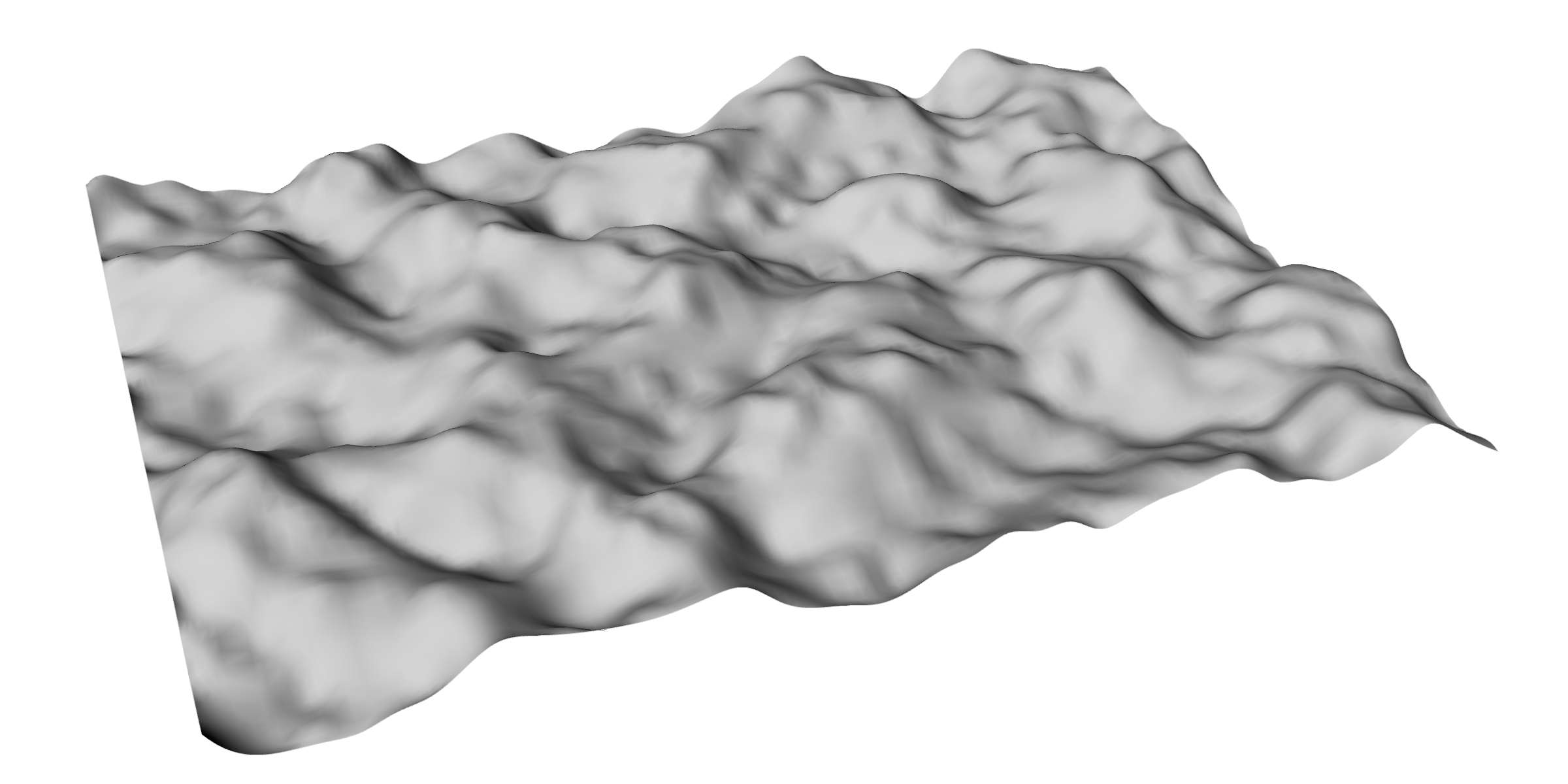
A heightmap created by layering multiple octaves of OpenSimplex noise.
Note
A completed, downloadable version of this example is available here:
../_static/grasshopper-files/simplex-heightmap.gh
Gradient noise is a type of noise that is perceptually “smoother” than noise generated by repeated PRNG calls alone. We won’t go into the math here, so don’t worry.
The first implementation of gradient noise was created by Ken Perlin, aptly named Perlin noise. It was originally developed to create procedural textures for the original Tron movie, but has since been used for procedural terrain and particle systems. Since its creation, other types of gradient noise, like fractal and simplex noise, have become incredibly popular.
For this example, we’ll be using OpenSimplex noise, which was created to get around the
patent Ken Perlin had registered for simplex noise. We’ll be using it to create a 2.5D
height map, similar to what we had done when first learning about Randomized Height Maps. To do this, we’ll be installing the opensimplex library.
Creating a new Grasshopper file, we can create a new Python 3 component:
Inputs:
point: type-hinted to Point3d, set to Item Accessseed: type-hinted to int, set to Item Access
Outputs:
point: type-hinted to Point3d
Inside, we can include the following code:
# r: opensimplex

import opensimplex
if seed is not None and isinstance(seed, int):
    # This check is just to make sure we don't crash Rhino if the seed input isn't connected
    opensimplex.seed(seed)
point.Z = opensimplex.noise2(point.X, point.Y)
Now that we have this, we can connect a Square grid component into the point input,
connect a slider into the seed input, and use a Surface from Points component
from the point output.
Important
When using the Surface from Points component on the point output, make sure the
Points input is flattened, and pass 1 more than the Extent X used for the Square grid
component into the U Count input.
Adding Octaves
A common practice with creating procedural textures and terrain with gradient noise is layering multiple “octaves” on top of each other. What this looks like is you generate multiple noise values for each point in the grid and add them together, but the noise generated has smaller and smaller amplitude, and the apparent size of high and low patches gets smaller and smaller as you add in more terms.
What this looks like is:
Where \(A_i\) are the amplitudes and \(f_i\) are the “frequencies” of your chosen layers. Higher frequencies mean smaller patches. These are called octaves because normally, it’s good to choose a base frequency and then layer in noise generated at integer multiples of that base frequency (like octaves for sound waves).
To support this, we need to add 2 more inputs to the Python script:
frequencies: type-hinted to float, set to List Accessamplitudes: type-hinted to float, set to List Access
Important
It’s incredibly important that these are set to List Access. If you don’t do that, this won’t work.
We can update the code, too:
# r: opensimplex

import opensimplex
if seed is not None and isinstance(seed, int):
    # This check is just to make sure we don't crash Rhino if the seed input isn't connected
    opensimplex.seed(seed)

for freq, amp in zip(frequencies, amplitudes):
    point.Z += amp * opensimplex.noise2(point.X * freq, point.Y * freq)
Now, to control the amplitudes and frequencies, we can use a bunch of sliders, fed into
two Merge components, fed into these two new inputs. Note that the
zip() function will pair up items in the input lists until one
is exhausted, so if you have frequencies than amplitudes, it will stop short once
all amplitudes are used.
Using gradient noise with multiple layers can give you incredibly fine-grained control over a heightmap’s generation, which can allow you to create fairly realistic terrain. Combining layers in other ways, such as having amplitudes that increase near an attractor point to get the semblance of a mountain, can give even more control.