Assignment 4: Elementary Cellular Automaton

Due: Friday, March 7, 2025

Important

Download the template Grasshopper document here: A4 Boilerplate.

Context

During Week 8, we introduced Cellular Automata, contextualized with Conway’s Game of Life, showing how something so separated from design can make for interesting geometry when framed in the right way. For this assignment, we’ll be doing something similar, but using much a simpler, 1-dimensional cellular automaton. With this, instead of converting the grid to cubes and stacking generations on top of each other, each generation is a \(1 \times n\) grid that we can stack on top of each other to make a \(m \times n\) image.

Rules

In the Game of Life, a cell in the grid is updated by checking its state and the states of its Moore neighborhood. In an elementary cellular automaton, the neighborhood of any cell are the two cells to its left and right. This means the rules that we could devise are based on the states of the cell itself and its two neighbors. For this assignment, there are only two valid states (“on” and “off”, \(0\) or \(1\)), which means there are \(2^3 = 8\) possible configurations for a cell and its neighborhood. Given one of these configurations, we could either choose to say that a state with that configuration will be either on or off in the next generation, meaning there are \(2^8 = 256\) possible rules for the type of elementary cellular automata we’re making in this assignment.

An example rule is: \(0, 1, 1 \rightarrow \text{True}\), meaning if the left neighbor of the cell is off, the cell itself is on, and its right neighbor is on, in the next generation, the cell will be on. The opposite rule would be \(0, 1, 1 \rightarrow \text{False}\), where given the exact same configuration in the current generation, the cell would be off in the next generation.

An example of how a set of rules are applied to a current generation. The rules are depicted as a 3-cell neighborhood above what the state of the center cell will be in the next generation.

Credit: Cormullion, CC BY-SA 4.0, via Wikimedia Commons.

Boundary Conditions

As with the Game of Life, elementary cellular automata exist on an infinite grid. Unfortunately for us, we can’t really do this very well. Instead, we can only work with a finite 1-dimensional grid. For the cell at the very beginning or the cell at the very end, their neighborhood can’t be directly found, so we need to come up with some way to provide it with fake information about its neighborhood. This gives us a handful of possibilities for what to use as the value for the missing neighbor:

1. Zero: treat the missing neighbor as being off (having a value of \(0\)).

2. One: treat the missing neighbor as being on (having a value of \(1\)).

3. Wrap: treat the missing neighbor as having the same state as the cell on the other boundary, as if the grid were a connected ring.

4. Extend: treat the missing neighbor as having the same state as this cell.

You’ll be able to choose the boundary conditions for both the left and right boundaries of the grid.

First Generation Type

The first generation can be one of many options:

1. Left 1: every cell is off except for the leftmost.

   

   

2. Centered 1: every cell is off except for the center cell.

   

   

3. Right 1: every cell is off except for the rightmost.

   

   

4. Left 0: every cell is on except for the leftmost.

   

   

5. Centered 0: every cell is on except for the center cell.

   

   

6. Right 0: every cell is on except for the rightmost.

   

   

7. Randomized: each cell is given a random state.

   

   Created with seed: 320

   

   Created with seed: 320

Technically, you could curate the first generation to have a specific configuration, but the boilerplate doesn’t provide this option on its own. You’d have to change the provided code in order for this to work.

Configuration

Parameters Group

• Length: the length of the 1-dimensional grid to use (snaps to odd values).

• Generation Count: the number of generations to include in the output.

• Value at Left Boundary: left boundary condition (see above).

• Value at Right Boundary: right boundary condition (see above).

• First Generation Type: the type of configuration to use as the first generation (see above).

• Seed: if using a Randomized first generation, the seed to use for the random number generator.

Rule Selection Group

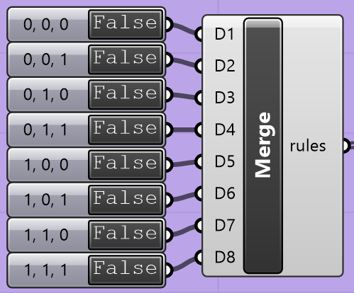
You have two options for creating the list of rules to use when calculating generations. The first way is to use the toggle switches that get passed into a Merge component, which is then provided to the rules parameter of the Python 3 Script component. These toggle switches are named with the configuration of a cell and its neighborhood at the current generation, with the True or False value being used to determine the state of that cell at the next generation. For example, the toggle switch named 0, 1, 1 determines the state of a cell if, in the previous generation, it was turned on, its left neighbor was off, and its right neighbor was on. If the switch is set to True, it will be on; if set to False, it will be off.

Alternatively, below these toggle switches, you could set the number in the slider to a number between 0 and 255 and connect the output of the Python 3 Script component the slider is connected to into the rules parameter of the main Python 3 Script component. As mentioned earlier, there are 256 possible sets of rules for an elementary cellular automaton, and this lets you choose the number directly. If you’d like to see a preview of what these can look like, there’s a helpful graphic on Wikipedia that connects the rule number to what the output would look like on an infinite grid with the first generation set equivalently to “Centered \(1\)“. Note that these are demonstrated on an infinite grid, which means your output will probably look a little different because you have to worry about boundary conditions.

Rendering Options Group

• Cell Size: the side length (in model units) of the grid cells.

• Surface Scale: the scale of the surfaces created relative to the size of the grid cells. If this is less than 1, there will be gaps between the created surfaces. You’ll get weird results setting this greater than 1, but it’s kind of cool to see, particularly at values around 1.5.

• On Color: the color to use for cells that are on.

• Off Color: the color to use for cells that are off.

Example

The image at the top of the page was created with the following configuration:

• Length: 75

• Generation Count: 45

• Value at Left Boundary: One

• Value at Right Boundary: One

• First Generation Type: Centered 1

• Seed: N/A

• Rule: 105 (from top to bottom: True, False, False, True, False, True, True, False)

• Cell Size: 1

• Surface Scale: 0.95

Task Description

In the template Grasshopper file above, you will edit the Python 3 Script node titled “Compute Generations”. The node itself will be red, and it’s contained in a group with the caption “Implement Me!”

Type Aliases

As with Assignment 3, I’ve provided you with some type aliases that are meant to make type hints easier to understand. The following aliases are provided to you:

type CellState = Literal[0, 1]

A cell’s state can either be off (0, False) or on (1, True).

type Neighborhood = tuple[CellState, CellState, CellState]

A cell’s neighborhood is represented as a 3-tuple, (a, b, c), where a is the state of its left neighbor, b is its own state, and c is the state of its right neighbor.

type Generation = Sequence[CellState]

Each generation is represented as a sequence of states representing the entire grid.

Important

These values are only used for type hints on variables and functions. It’s good practice to not use these names as variables because you can confuse a static type checker or yourself.

These aliases are important so I can explain in these instructions what you need to do without having to spell everything out.

Helpful Data

You are provided with some variables that you might find helpful:

rules: dict[Neighborhood, CellState]

A map from Neighborhoods to CellStates, where the value at a given Neighborhood the CellState to use in the next Generation for a cell with that Neighborhood in the current Generation.

length: int

The length of the 1-dimensional grid.

num_generations: int

The number of generations to compute, including the first.

Helper Functions

You are provided with three functions that you might find helpful:

left_boundary_behavior(gen: Generation) → CellState

Provides the value to use as the left neighbor’s CellState for the leftmost cell in the grid.

Parameters:

gen – The current Generation.

Returns:

The CellState to use, determined by the left_boundary_condition component input.

right_boundary_behavior(gen: Generation) → CellState

Provides the value to use as the right neighbor’s CellState for the rightmost cell in the grid.

Parameters:

gen – The current Generation.

Returns:

The CellState to use, determined by the right_boundary_condition component input.

get_first_generation() → Generation:

Computes and returns the first Generation.

Returns:

The first Generation, determined by the first_generation_type component input.

Things to Implement

Inside the script, scroll down to the “Implementation” section. Here, you’ll be implementing four functions:

get_neighborhood(gen: Generation, index: int) → Neighborhood

Compute the Neighborhood of the grid cell at the provided index.

Parameters:

• gen – The current Generation.

• index – The index of the grid cell to compute the Neighborhood of.

Returns:

The Neighborhood of the grid cell at the provided index.

Implementation Details

1. Return a 3-tuple: (gen[index - 1], gen[index], gen[index + 1])

2. If index == 0, use left_boundary_behavior(gen) instead of gen[index - 1].

3. If index == length - 1, use right_boundary_behavior(gen) instead of gen[index + 1].

Important

It’s incredibly important that you output a tuple here, and not something else. If you don’t, your implementation of next_state() won’t work.

next_state(gen: Generation, index: int) → CellState

Compute the next Generation‘s CellState of the grid cell at the provided index.

Parameters:

• gen – The current Generation.

• index – The index of the grid cell to compute the next CellState of.

Returns:

The next CellState of the grid cell at the provided index.

Implementation Details

1. Compute the Neighborhood of gen[index] using the get_neighborhood() function.

2. Get the CellState corresponding to the computed Neighborhood. This can be done by accessing rules with the Neighborhood as the key.

3. Return the CellState determined in the previous step.

next_generation(gen: Generation) → Generation

Compute the Generation following a provided Generation.

Parameters:

gen – The current Generation.

Returns:

The next Generation.

Implementation Details

Create a new sequence (tuple or list) according to the following:

1. For each index in range(length):

   1. Compute the next_state() for the cell at that index.

   2. Include the computed CellState in your output Generation.

generate() → list[Generation]

Compute all Generations, returning the list of computed Generations.

Returns:

A list of computed Generations.

Implementation Details

1. Create an empty list called generations.

2. Compute the first Generation with get_first_generation() and save it to a variable called gen.

3. Loop over range(num_generations), doing the following for each iteration:

   1. Append gen to generations.

   2. Update gen with the output from next_generation().

4. Return generations.

Tips

1. As you’re debugging, I suggest using only a single rule set to True. This should help you determine if your implementation makes sense.

   • Recall what each rule means, and it should make it more clear whether your implementation is correct or not.

2. As you’re debugging, you’ll probably want to switch around your First Generation Type while setting a single rule to True because some of the rules won’t do anything with Centered 1.

3. Correctness is highly important for this assignment due to its simplicity. You definitely want to make sure each rule works on its own.

   • You’ll also want to make sure that your boundary conditions work as expected, as well.

Submission

A Note on Correctness

Correctness is hugely important for this assignment. If your implementation does not produce exactly the same thing as mine, you have implemented something incorrectly.

As such, you will need to include the configurations you used when producing your graphics.

Deliverables

When submitting your assignment, upload a .gh file containing your solution. Also create a handful of pictures (minimum 5) showcasing the rigorousness of your solution. With each image, include either a text description or a picture of the configuration you used to generate them (see the above example). There are some constraints on the types of configurations you can use when creating your pictures:

• Only one of your pictures may have less than two rules set to True.

  • If using the slider, only one of your pictures can be created with one of 0, 1, 2, 4, 8, 16, 32, 64, or 128.

• You must showcase each of the boundary conditions for the left and right boundaries. You can mix and match as much as you like.

  • At a bare minimum, you could set both boundary conditions to the same value, choosing one value per image. Your fifth image can then use whatever you’d like as the boundary conditions.

These constraints ensure that your pictures demonstrate the completeness of your implementation.

Rubric

Points	Requirements
30	You have created at least 5 pictures showcasing the rigorousness of your solution, and you have included the configurations used to generate them.
30	The configurations used to create your pictures adhere to the constraints outlined in the Deliverables section.
10	Your implementation of get_neighborhood() correctly computes the Neighborhood of any given cell index in any given gen, including the boundary conditions.
10	Your implementation of next_state() correctly computes the next CellState of any given cell index in any given gen with any given rules, based on your implementation of get_neighborhood().
10	Your implementation of next_generation() correctly computes the next Generation of any given gen, based on your implementation of next_state().
10	Your implementation of generate() correctly provides a list of num_generations Generations, starting with the first generation calculated by get_first_generation(), with each Generation afterwards being calculated by your implementation of next_generation().

Note

The implementation requirements are all based on the previous implementation requirement. This means that even if your implementation of one function is incorrect, if you’re calling it correctly in the appropriate function, you’ll get full credit for the calling function.